
Bearing fault detection with vibration analysis.
Find a rolling bearing defect in an accelerometer recording with envelope analysis: band-pass, rectify, low-pass, FFT, and checks at BPFO, BPFI and BSF. A downloadable LazyAnalysis graph, built by AI through MCP and independently validated.
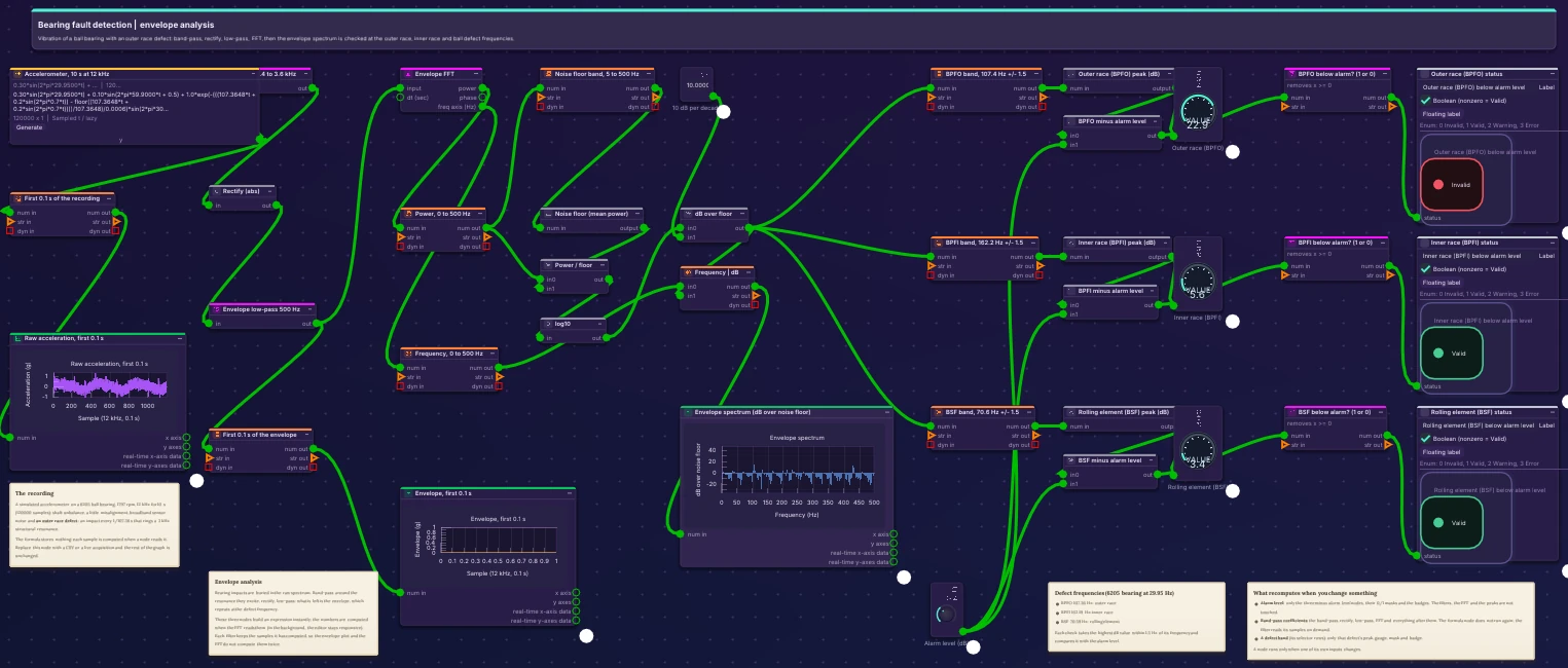
Accelerometer → Band-pass → |x| → Low-pass → FFT → dB over floor → BPFO · BPFI · BSF → Alarm
38 nodes · 120000 samples · opens on its dashboard · notes in the node editor explain each stage
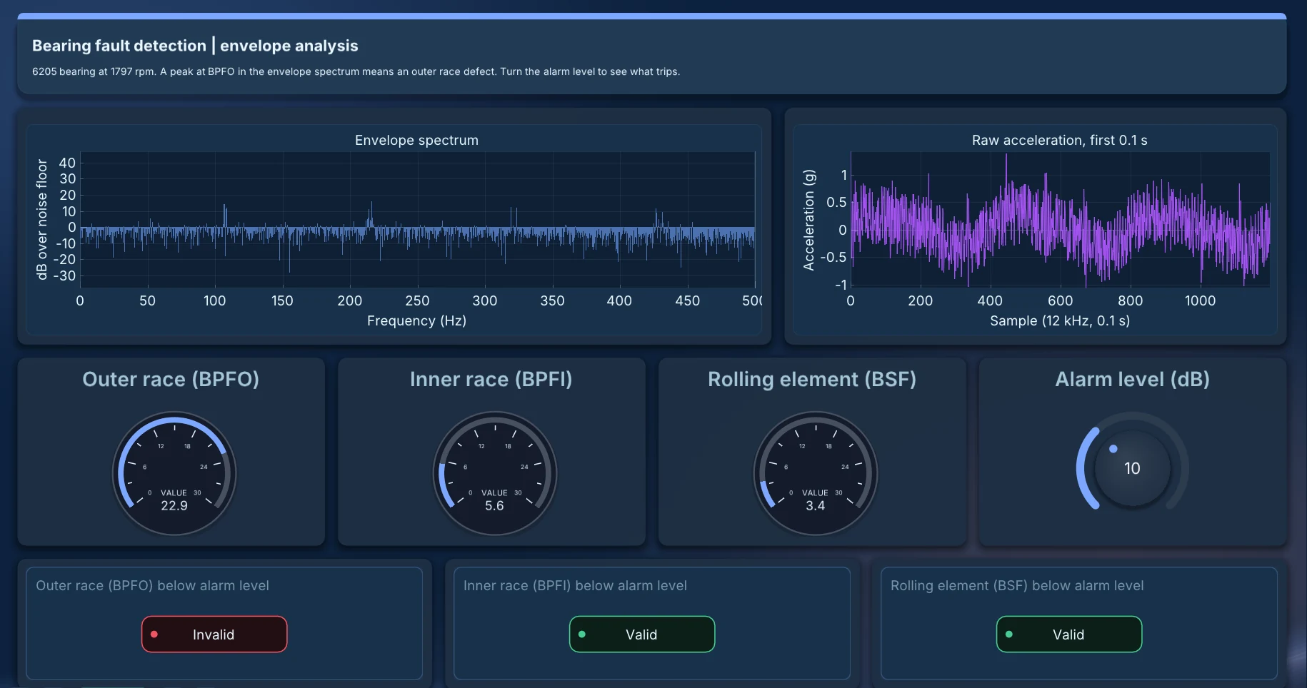
| Defect | Frequency | Peak over the noise floor | At a 10 dB alarm level |
|---|---|---|---|
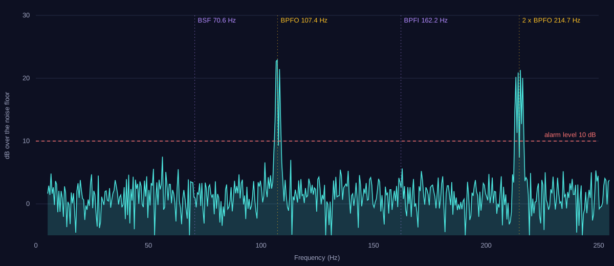
| Outer race (BPFO) | 107.36 Hz | 22.9 dB | Alarm |
| Inner race (BPFI) | 162.19 Hz | 5.6 dB | Below |
| Rolling element (BSF) | 70.59 Hz | 3.4 dB | Below |
“Build a LazyAnalysis graph that finds bearing defects in a 12 kHz accelerometer recording of a 6205 bearing at 1797 rpm: envelope analysis around the 3 kHz resonance, the envelope spectrum in dB over its noise floor, checks at BPFO, BPFI and BSF, and a dashboard with an alarm level I can turn.”
How to connect your assistant ↗The problem
A rolling bearing with a damaged outer race hits the damage at a fixed rate: the ball pass frequency of the outer race (BPFO), 3.58 times the shaft speed for a 6205 bearing. Each hit is short and weak. It rings a structural resonance of the machine, and in the raw spectrum it is buried under shaft unbalance and noise. Envelope analysis recovers it, and it is the standard first check in vibration-based condition monitoring.
The graph
A simulated accelerometer on a 6205 ball bearing at 1797 rpm, sampled at 12 kHz for 10 seconds (120000 samples), with an outer race defect. The signal is band-passed around the 3 kHz resonance (2nd order Butterworth, 2.4 to 3.6 kHz), rectified and low-passed at 500 Hz: what is left is the envelope, which repeats at the defect frequency. Its FFT is shown in dB over its noise floor and checked within 1.5 Hz of the outer race, inner race and rolling element frequencies. The dashboard has the spectrum, the raw signal, a gauge per defect, an alarm level knob and a badge per defect. Replace the simulated source with a CSV file or a live acquisition and the rest of the graph is unchanged.
What recomputes when you change something
LazyAnalysis pushes a change downstream only: a node runs when one of its own inputs changes. Turn the alarm level: only the three comparisons, their 0/1 masks and the badges run again; the filters, the FFT and the peaks are not touched. Change the band-pass: the filters, the FFT and everything after them run again, while the source does not, since it stores no samples and the filter reads them on demand. Change one defect band: only that defect's peak, gauge and badge.
Lazy evaluation, caching and the background
The filters and the rectifier build expressions without computing anything. The samples are computed when the FFT reads them, in a background job, so the editor stays responsive. Each IIR filter keeps the samples it has computed, so the envelope plot and the FFT do not compute them twice. The file carries its own notes that say all of this next to the nodes.
Built by AI, checked independently
The graph was built by an AI assistant (Claude) sending a description of the nodes, links, notes and dashboard to the LazyAnalysis MCP server, which wrote and validated the file. It was then checked three ways: the analysis written directly in NumPy and SciPy, the nodes of the file run with NumPy following the file's own links and settings, and the LazyAnalysis engine code run on the file's settings. All three give the results above; the engine's envelope matches SciPy within 1e-11. Building this example also found and fixed three problems in the engine: two in the speed of the IIR filter, and one in how a node gets an input that a background job delivers late.